Picture a small software agent in a simulated corridor. Its picture of the world says the door ahead will stay shut. It walks through anyway. Something in its model is wrong, and it has to work out what.
We study this kind of situation as part of a research program at FriendMachine on what we call field intelligence. One question we care about is whether an agent’s model of its world can run entirely as local updates, where each small piece of the model only ever talks to its immediate neighbors. Doing that means translating, or compiling, a set of rules into a network of such updates. In a small experiment built around the corridor above, we found that the translation hides choices that change the answers you get.
The central one is this. Two models can describe exactly the same behavior and still be very different to compute with. In one version, simple local updates might give exact answers. In the other, they might only approximate. What separates them is how the model is split into rules, and that choice deserves as much scrutiny as the rules themselves.
The setup: a corridor, a key and two doors
The test world is a small, deterministic toy, deliberately tiny. The agent moves along a short corridor containing a key and two doors. It can step left or right, pick up or drop the key, or wait. Its starting model is wrong. The model predicts that a door will stay shut, and then the agent walks through it. The agent has to work out why its model failed and fix it.
We wrote the agent’s world model as a set of local rules, compiled it into a network that updates beliefs by passing messages between neighbors, and repaired the model when it turned out to be wrong. To follow what we learned, you need two ideas about how such networks work.
From rules to messages
A factor graph is a diagram of a model. Circles stand for variables, such as the agent’s position or whether it is holding the key. Squares stand for rules, called factors, that link the variables they involve. A rule might say “the agent can pass the door only if the door is passable.”
Message passing answers questions about the model, such as “where is the agent likely to be?”, using only local steps. Each variable and each rule repeatedly sends a short summary of what it knows to its direct neighbors. When the graph is a tree, meaning it has no loops, this gives exact answers. When the graph has loops, messages circulate around them and the result is an approximation. The messages can settle on stable values that are still wrong, so settling down does not by itself mean the answer is right.
Whether the graph has loops therefore matters a great deal, and it turned out to depend on choices that can look like mere formatting.
Lesson 1: the same rules can make a tree or a loop
We wrote the same world two ways, with the same transition behavior in both. A transition rule says how each part of the state changes from one step to the next.
In the first version, each next-step variable depends only on what actually affects it. Whether the agent holds the key next step depends on whether it holds the key now and what it does. Its next position depends on its current position and on whether the door is passable. Written this way, the model compiles to a tree, and each rule involves at most three variables.
In the second version, every next-step variable reads the whole previous state. That is a natural way to translate a simulator mechanically, and it changes no behavior. But now several rules share the same inputs, those shared inputs close loops, and the largest rule involves four variables. Simple message passing on this version is only approximate.
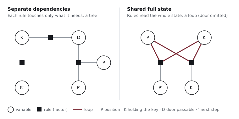
You can handle the loop in three ways, and each has a cost. Keeping many small rules often gives a tree, but you have to know which dependencies are real. Merging the shared state into one large rule keeps answers exact, but the messages grow exponentially. Grouping variables into clusters with standard techniques, such as junction trees, also works, though the size of each group is a cost that has to be reported.
Compiling a model into local updates therefore involves a decision about how to split it. That decision is part of the science, and the compiler, the program that does the translation, should report what it chose.
Lesson 2: what you observe can change the shape of the problem
Once we saw that the split decides exactness, it was tempting to label a whole model “exact” or “approximate.” That turned out to be wrong too.
Conditioning means fixing some variables to the values you actually observed, and observations change the graph. A sensor reading that nobody looked at can be dropped without affecting any answer. Observing a relationship between two things, such as where the key is relative to the agent, adds a rule that ties those two parts of the model together. That new link can join branches that were separate and create a loop.
Exactness belongs to the graph after conditioning on the evidence. The same model can be exact for one set of observations and approximate for another, and every result needs to say which it was.
Lesson 3: a fix comes as a bundle
So far the model has been fixed. The other half of the experiment was changing it, which brings us back to the door the agent should not have been able to pass.
The correct explanation for the surprising door was that the agent was carrying the key, and the original model had no variable for that. It is tempting to call the fix “add one yes/no variable,” but that alone does not produce a working model. The repair needed several pieces at once:
- the new “holding the key” variable
- where the key is when the agent is not holding it
- what picking up and dropping do
- the door’s dependence on holding the key
- how existing states carry over to the new model
Leave out a piece and the model is incomplete or inconsistent. We therefore treat a repair as a complete, self-consistent bundle: the full new model plus an exact list of what changed. Testing an alternative explanation works the same way. It needs the earlier steps, such as when the agent picked up the key, as well as the single step where the prediction failed.
Lesson 4: experiments often beat watching
“Carrying the key” was the right answer, but the agent did not know that at the start. It began with four candidate explanations:
- holding the key lets you through doors
- touching the key unlocks doors permanently
- the key works only once and is then used up
- a counting rule that depends on earlier attempts at the doors
Watching more ordinary behavior often cannot separate them. Walking through the second door while still holding the key fits both “holding the key” and “permanent unlock.” An experiment that acts on the suspected cause can do better. Dropping the key and then trying the second door gives a different, visible outcome under each remaining explanation.
How much such an experiment teaches depends on what the agent can observe. We measure that in bits. One bit is what you learn from the answer to a fair yes-or-no question, so telling apart four equally likely options takes 2 bits. In the default setup, what the agent saw of the key in the earlier steps already rules out the counting rule. Three explanations remain, and the experiment separates all three. With each equally likely beforehand, that is log₂ 3, about 1.585 bits of information.
In a variant where the agent sees only its own movement, nothing rules out the counting rule early. All four explanations remain, and a slightly different five-step experiment separates them, which is exactly 2 bits. A claim like “this experiment is worth 2 bits” is incomplete until it says what the agent could see.
Limits of this example
All four lessons come from one very small world, so they are observations to test further rather than general results. This is a small, deterministic toy. The corridor has eight cells, the agent has five actions, and the four candidate explanations come from a list we wrote by hand rather than one the agent discovered. The compiler’s checks compared exact answers on about two hundred distinct situations. That covers this tiny world thoroughly and says nothing about larger ones. Nothing here shows that every rule system can be split into a tree, that the approach scales, or that local updates save energy.